Firm costs + profit maximization
Imagine a firm that produces chocolate milk using milk, cocoa powder, sugar, a spoon, a pot, and a refrigerator. The costs for creating different amounts of milk are all included in the Excel file below (and a finished version with all the decompositions and calculations is also included below).
Let’s use microeconomic principles to find out how much milk this firm should create if they want to maximize their profits and make the most money possible. Along the way we’ll decompose their costs into fixed and variable costs, marginal costs, and average costs. Finally we’ll find the elasticity of demand for chocolate milk to see how responsive consumers are to changes in chocolate milk prices.
Because this is a foundational microeconomic principle, there are billions of YouTube videos out there with tutorial about how to calculate these things. You should check these out for additional reference and help:
- Jacob Clifford, “Short-Run Costs (Part 1)"
- Jacob Clifford, “Short-Run Costs (Part 2)"
- Jacob Clifford, “Maximizing profit”
- Jacob Clifford’s entire production, cost, and perfect competition unit
- Khan Academy, “Fixed, Variable, and Marginal Cost”
- Khan Academy “Visualizing average costs and marginal costs as slope”
- Jodi Beggs, “Calculating and graphic the costs of production”
- Jodi Beggs, “Cost curves, economic profit, and supply”
- Jodi Beggs, “Profit maximization”
- Economicsfun, “How to Calculate Total Cost, Marginal Cost, Average Variable Cost, and ATC”
We’ll do this with both Excel and with math formulas. These videos walk through how to do it both ways, and the text below provides more step-by-step instructions.
Finding the cheapest cost of production
Cost function
Here are the firm’s costs at different levels of production:
| Quantity | Milk | Sugar | Chocolate powder | Spoon | Pot | Fridge |
|---|---|---|---|---|---|---|
| 0 | $0 | $0.00 | $0.00 | $1 | $4 | $15 |
| 1 | $2 | $0.50 | $0.10 | $1 | $4 | $15 |
| 2 | $6 | $1.50 | $0.30 | $1 | $4 | $15 |
| 3 | $12 | $3.00 | $0.60 | $1 | $4 | $15 |
| 4 | $20 | $5.00 | $1.00 | $1 | $4 | $15 |
| 5 | $30 | $7.50 | $1.50 | $1 | $4 | $15 |
| 6 | $42 | $10.50 | $2.10 | $1 | $4 | $15 |
| 7 | $56 | $14.00 | $2.80 | $1 | $4 | $15 |
| 8 | $72 | $18.00 | $3.60 | $1 | $4 | $15 |
| 9 | $90 | $22.50 | $4.50 | $1 | $4 | $15 |
| 10 | $110 | $27.50 | $5.50 | $1 | $4 | $15 |
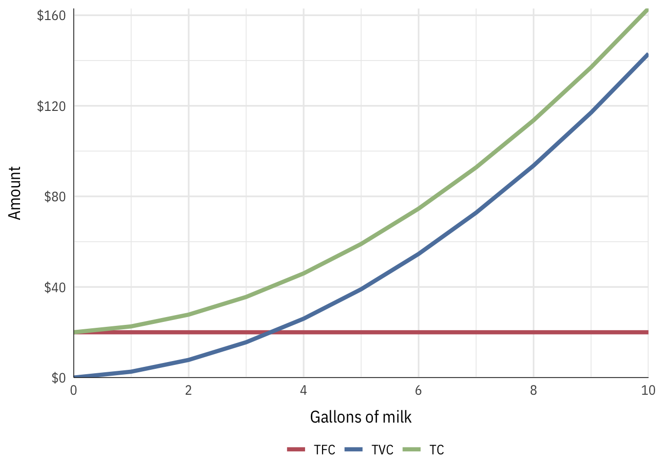
Total costs
We can divide these costs into fixed costs (spoon, pot, and fridge) and variable costs (milk, sugar, chocolate):
| Quantity | TFC | TVC | TC |
|---|---|---|---|
| 0 | $20 | $0.00 | $20.00 |
| 1 | $20 | $2.60 | $22.60 |
| 2 | $20 | $7.80 | $27.80 |
| 3 | $20 | $15.60 | $35.60 |
| 4 | $20 | $26.00 | $46.00 |
| 5 | $20 | $39.00 | $59.00 |
| 6 | $20 | $54.60 | $74.60 |
| 7 | $20 | $72.80 | $92.80 |
| 8 | $20 | $93.60 | $113.60 |
| 9 | $20 | $117.00 | $137.00 |
| 10 | $20 | $143.00 | $163.00 |
If we decompose total costs into fixed and variable costs, we see that the rise in costs is driven almost entirely by increasing variable costs.
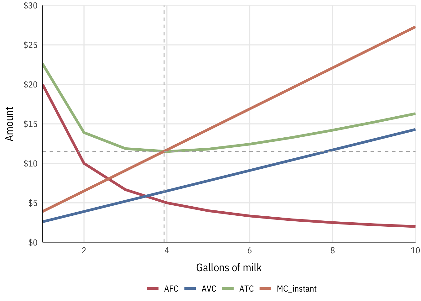
Average and marginal costs
We can find average costs by dividing the cost by the number of gallons of milk produced, and we can find the marginal cost by subracting the cost of the previous amount:
| Quantity | TC | AFC | AVC | ATC | MC_chunk | MC_instant |
|---|---|---|---|---|---|---|
| 0 | $20.00 | — | — | — | — | $1.30 |
| 1 | $22.60 | $20 | $2.60 | $22.60 | $2.60 | $3.90 |
| 2 | $27.80 | $10 | $3.90 | $13.90 | $5.20 | $6.50 |
| 3 | $35.60 | $7 | $5.20 | $11.87 | $7.80 | $9.10 |
| 4 | $46.00 | $5 | $6.50 | $11.50 | $10.40 | $11.70 |
| 5 | $59.00 | $4 | $7.80 | $11.80 | $13.00 | $14.30 |
| 6 | $74.60 | $3 | $9.10 | $12.43 | $15.60 | $16.90 |
| 7 | $92.80 | $3 | $10.40 | $13.26 | $18.20 | $19.50 |
| 8 | $113.60 | $2 | $11.70 | $14.20 | $20.80 | $22.10 |
| 9 | $137.00 | $2 | $13.00 | $15.22 | $23.40 | $24.70 |
| 10 | $163.00 | $2 | $14.30 | $16.30 | $26.00 | $27.30 |
The optimal (minimum) point on the ATC curve occurs when Q = 3.93. This is also not coincidentally where the MC curve intersects the ATC curve. The optimal price at this quantity is $11.52 per gallon of milk, but the firm won’t necessarily be able to set the price at that point on its own (unless it’s a monopoly; and even then, they’ll set it higher).
IMPORTANT NOTE: Because we’re dealing with curves and not lines, calculating marginal values with Excel by subtracting the previous value from the current value will not be 100% accurate. The only way to get perfectly accurate marginal values is to use calculus to find the instantaneous derivative at exactly that point.
Finding the optimal price and quantity
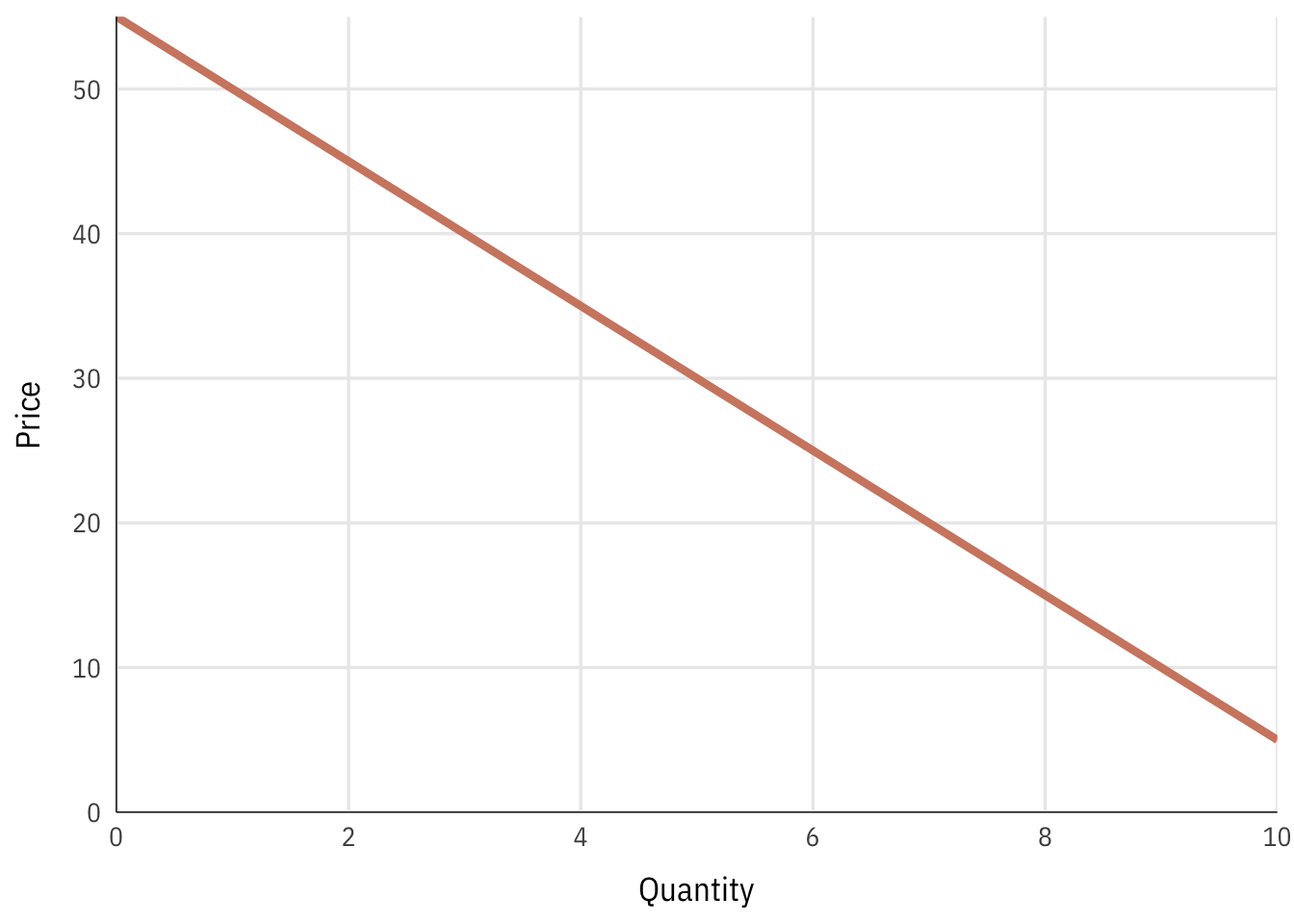
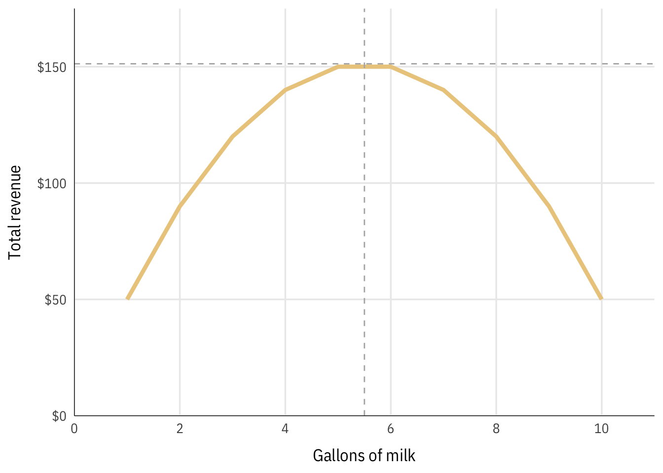
The firm’s quantity decision depends on the market demand for chocolate milk. The demand curve for this market looks like this:
With this demand curve, we can find the price and quantity that would produce the maximum revenue, assuming there were no costs to production.
| Quantity | Price | TR |
|---|---|---|
| 0 | $55 | $0 |
| 1 | $50 | $50 |
| 2 | $45 | $90 |
| 3 | $40 | $120 |
| 4 | $35 | $140 |
| 5 | $30 | $150 |
| 6 | $25 | $150 |
| 7 | $20 | $140 |
| 8 | $15 | $120 |
| 9 | $10 | $90 |
| 10 | $5 | $50 |
The firm can maximize its revenue by producing 5.5 gallons of milk, which would create $151.25 in revenue.
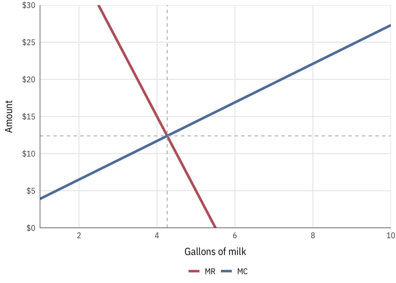
However, this doesn’t take into account the firm’s costs. The firm’s profit maximizing point is defined as \(MC = MR\), so we need compare marginal costs and marginal revenues and calculate total profit (π) across all quantities of output.
Again, note that using chunky marginal values by subtracting previous values won’t be as accurate as calculus-based instant marginal values.
To get correct marginal values we can find the formula for the total cost function by using Wolfram Alpha. If you make a list of all the points in the quantity and total cost columns (i.e. {{0, 20}, {1, 22.6}, {2, 27.8}}), you can fit a polynomial formula to those points with Wolfram Alpha.
For example, search for “quadratic fit {0, 20}, {1, 22.6}, {2, 27.8}, {3, 35.6}, {4, 46}, {5, 59}, {6, 74.6}, {7, 92.8}, {8, 113.6}, {9, 137}, {10, 163}" and you’ll see that the best formula for total cost is \(y = 1.3x^2 + 1.3x + 20\).
The marginal cost is the first derivative of the total cost, or \(y = 2.6x + 1.3\).
To find the equation for total revenue we need to multiply the demand function by Q (or x), since the formula for total revenue is \(TR = PQ\). By looking at the demand curve above, we can see that the y-intercept is 55 and the slope is −5, giving us \(y = -5x + 55\), or \(P = -5Q + 55\). We can find the total revenue formula with some algebraic trickery, substituting the \(P\) formula into \(TR = PQ\):
$$
\begin{aligned} TR &= PQ \\ &= (-5Q + 55)Q \\ &= -5Q^2 + 55Q \end{aligned}
$$
The total revenue formula is thus \(P = -5Q^2 + 55Q\).
The marginal revenue is the first derivative of the total revenue, or \(P = -10Q + 55\).
We can set MR and MC equal to each other to find the optimal x (or Q) ($2.6Q + 1.3 = -10Q + 55$), solve for x, and then plug that x into one of the total equations to find the optimal price.
The point where \(MC = MR\) can’t be seen in the table, since it happens between 4 and 5 gallons. If the firm produces 4.26 gallons of milk at a price of $12.38 per gallon, it will achieve its maximum profit of $94.43.
| Quantity | Price | TR | TC | MR_chunk | MR_instant | MC_chunk | MC_instant | π |
|---|---|---|---|---|---|---|---|---|
| 0 | $55.00 | $0.00 | $20.00 | — | $55.00 | — | $1.30 | -$20.00 |
| 1 | $50.00 | $50.00 | $22.60 | $50.00 | $45.00 | $2.60 | $3.90 | $27.40 |
| 2 | $45.00 | $90.00 | $27.80 | $40.00 | $35.00 | $5.20 | $6.50 | $62.20 |
| 3 | $40.00 | $120.00 | $35.60 | $30.00 | $25.00 | $7.80 | $9.10 | $84.40 |
| 4 | $35.00 | $140.00 | $46.00 | $20.00 | $15.00 | $10.40 | $11.70 | $94.00 |
| 4.262 | $33.69 | $143.59 | $49.15 | $17.38 | $12.38 | $11.08 | $12.38 | $94.43 |
| 5 | $30.00 | $150.00 | $59.00 | $10.00 | $5.00 | $13.00 | $14.30 | $91.00 |
| 6 | $25.00 | $150.00 | $74.60 | $0.00 | -$5.00 | $15.60 | $16.90 | $75.40 |
| 7 | $20.00 | $140.00 | $92.80 | -$10.00 | -$15.00 | $18.20 | $19.50 | $47.20 |
| 8 | $15.00 | $120.00 | $113.60 | -$20.00 | -$25.00 | $20.80 | $22.10 | $6.40 |
| 9 | $10.00 | $90.00 | $137.00 | -$30.00 | -$35.00 | $23.40 | $24.70 | -$47.00 |
| 10 | $5.00 | $50.00 | $163.00 | -$40.00 | -$45.00 | $26.00 | $27.30 | -$113.00 |
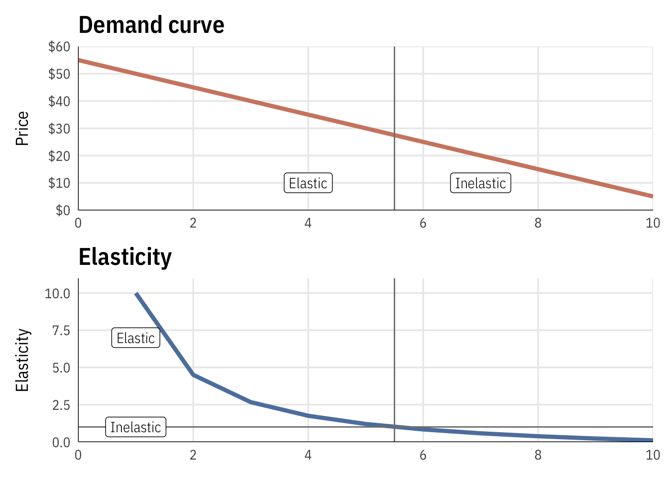
Elasticity of demand
Recall the formula for elasticity:
$$
\begin{align} \varepsilon &= -\frac{\% \text{ change in demand}}{\% \text{ change in price}} \\ &= - \frac{\% \Delta Q}{\% \Delta P} \end{align}
$$
Remember that \(\% \Delta Q = \frac{Q_{\text{new}} - Q}{Q}\) and that \(\% \Delta P = \frac{P_{\text{new}} - P}{P}\) (or just \(\frac{\text{new} - \text{old}}{\text{old}}\)). We can also write \(Q_{\text{new}} - Q\) as \(\Delta Q\), or just the change in \(Q\) (and also \(\Delta P\)). This means we can rewrite the equation like so:
$$
\begin{align} \varepsilon &= - \frac{\% \Delta Q}{\% \Delta P} \\ &= - \frac{\frac{Q_{\text{new}} - Q}{Q}}{\frac{P_{\text{new}} - P}{P}} \\ &= - \frac{\frac{\Delta Q}{Q}}{\frac{\Delta P}{P}} \end{align}
$$
We can then simplify this huge hairy fraction by multiplying both the numerator and denominator by the inverse of the denominator, \(\frac{P}{\Delta P}\):
$$
\begin{align} \varepsilon &= - \frac{\frac{\Delta Q}{Q}}{\frac{\Delta P}{P}} \times \frac{\frac{P}{\Delta P}}{\frac{P}{\Delta P}} \\ &= - \frac{\Delta Q}{Q} \times \frac{P}{\Delta P} \\ &= - \frac{\Delta Q}{\Delta P} \times \frac{P}{Q} \end{align}
$$
That’s the final version of the price elasticity of demand formula: \(\varepsilon = - \frac{\Delta Q}{\Delta P} \times \frac{P}{Q}\). Conveniently, \(\frac{\Delta Q}{\Delta P}\) is also the inverse slope of the demand curve.
| Quantity | Price | \(\frac{\Delta Q}{\Delta P}\) |
\(\frac{P}{Q}\) |
ε |
|---|---|---|---|---|
| 1 | $50 | -0.2 | 50 | 10 |
| 2 | $45 | -0.2 | 22.5 | 4.5 |
| 3 | $40 | -0.2 | 13.33 | 2.667 |
| 4 | $35 | -0.2 | 8.75 | 1.75 |
| 5 | $30 | -0.2 | 6 | 1.2 |
| 6 | $25 | -0.2 | 4.167 | 0.8333 |
| 7 | $20 | -0.2 | 2.857 | 0.5714 |
| 8 | $15 | -0.2 | 1.875 | 0.375 |
| 9 | $10 | -0.2 | 1.111 | 0.2222 |
| 10 | $5 | -0.2 | 0.5 | 0.1 |
Demand is elastic in the first half of the demand curve, and inelastic in the second half, as seen here: